Russian
Related work
Adaptive plotting and undersampling
Honest plotting
There exist countless programs on every platform to graph functions of one variable. Nearly all of them utilize what we shall refer to as the naive algorithm of linearly sampling the function at a predetermined number of equally spaced points and connecting those points with lines, after some scaling to fit all the points in a box. For functions of two variables, many systems will sample the function on a square grid of points, connect adjacent points with triangles, and render the surface with a 3D rendering package.
Adaptive plotting and undersampling
Most of the plotters included with CA systems use an adaptive sampling method for plotting of curves. They first sample the function at relatively few points and recursively calculate more points if adjacent points are not almost collinear. This is useful for curfes whose curvature varies sharply and for which the defining expressions are expensive to evaluate.
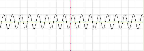
Figure1: A naive plot of sin(300x) in Graphing Calculator

Figure2: An adaptive plot of sin(300x) in Mathematica
In [Fat92], Fateman discusses failure modes due to undersampling. For instance, Figure 1 shows sin(300x) evaluated once per screen pixel in the Graphing Calculator. Although sine is a simple periodic function, we see in the plot an additionally layer or structure which is an artifact of the sampling showing us a beat frequency between the frequency of the function and the frequency of the pixels. Adaptive sampling does not help this failure mode although it does creat more interesting artificial structure as in Figure 2 of sin(300x) for [0,1] in Mathematica.
Some systems, rather that sample at linearly spaced coorinates, will add a small random jitter to each abscissa value. This replaces the false structure shown in Figure 1 and 2 with random noise which visually obviously requires a finer sampling.
Honest plotting
Consider 1+x 2+0.0125ln|1-3(x-1)|. Most systems will step over the narrow valley where the function diverges. In [Fat92], fateman describes a graphing method using interval arithmetic which he calls honest plotting. Interval arithmetic generalizes ordinary arithmetic to closed, bounded ranges of real numbers [Moo79]. Using interval arithmetic, it is possible to compute and plot rigorous error bounding regions and hence, be sure that the curve lies somowhere in that region. Interval arithmetic is now widely accepted within the graphics community as shown by the growing number of publications (see [Sny92] for instance).
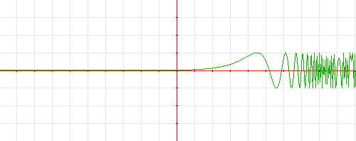
Figure3: An honest plot of sin(ex) in Graphing Calculator
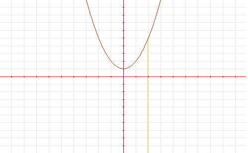
Figure4: An honest plot of 1+x2+0.0125ln|1-3(x-1)| in Graphing Calculator
Consider figure 3. It shows with sin(e x) that as the frequency of oscillation increases, rather that degenerate into noise or show a misleading beat frequency, the plot gradually becomes a solid band containing the function. Fifure 4 shows honest plotting catching the valley at x=4/3 in 1+x 2+0.0125ln|1-3(x-1)|.

Figure5: An honest plot of sinx/x in Graphing Calculator
Although the function is guaranteed to lie within the plot area, bounds can be quite pessimistic using honest plotting. For example, Figure 5 shows sinx/x plotted with intervals the width of one pixel using the natural interval extension of the function. The width of the curve near the origin arises because the correlation between the numerator and denominator is not taken into account in the natural interval evaluation. Although the actual curve is contained within the honest plot, the plot implies that the function may be oscillating wildly, or may diverge near the origin when in fact it is well-behaved. As suggested in [Fat92], honest plotting should be used together with other techniques for getting a true figure of a curve or surface.
Contents Back Next
|